LOG/Blog Post

Why Asynchronous Pipelines Don't Scale — and How a Rotation Fixes Them

An optimizer-side route towards bubble-free pipeline parallelism.

Authors

Hyunji Jung*, Sungbin Shin*, Namhoon Lee  — POSTECH

Paper

arXiv:2602.03515  ·  Code

Venue

International Conference on Machine Learning (ICML) 2026

Date

2026 May

§1Pipelines, bubbles, and a scaling failure

Train a large language model and you very quickly run out of memory. A 70-billion-parameter model's weights alone occupy 140 GB in half precision — already nearly twice what a single H100 holds. Gradients, Adam's two moment buffers, and activations push the training-time requirement past a terabyte. The model that does not fit on one device has to be partitioned.

So it has to be split across devices. Tensor parallelism and sharded data parallelism (ZeRO [1] / FSDP) can do that, but both rely on collective communication, where all the GPUs in a group exchange data at once: tensor parallelism all-reduces inside every layer, so it stays cheap only within a single node, and sharded data parallelism all-gathers the full weights on every step. Pipeline parallelism instead just passes only small activations and gradients, peer-to-peer, so it spans many nodes efficiently — which is why a frontier-scale model implies a deep pipeline.

Concretely, pipeline parallelism divides the layers into \(P\) contiguous groups (call each group a stage) and places each group on its own device. Each micro-batch's activations travel forward from stage 1 to stage \(P\), and its gradients then travel backward from stage \(P\) to stage 1. With multiple micro-batches in flight at once, devices can work in parallel — each on a different micro-batch in a different part of the forward or backward pass.

The classical, synchronous scheduling discipline — introduced by GPipe [2] — collects gradients from every micro-batch before any stage updates its weights. But this naive scheduling leaves devices idle — pipeline bubbles — results in severely suboptimal hardware utilization.

The alternative, proposed by PipeDream [3], drops the synchronization barrier. Each stage immediately updates its weights and starts the forward pass of the next micro-batch without waiting for others to finish their backward passes. The pipeline runs bubble-free.

In practice, this staleness is not minor — especially for deep transformers, the very regime asynchronous training was designed to enable. Since the delay \(\tau\) grows with pipeline depth, a larger model that requires a deeper pipeline produces larger staleness, fundamentally undermining the scalability the method was designed to provide.

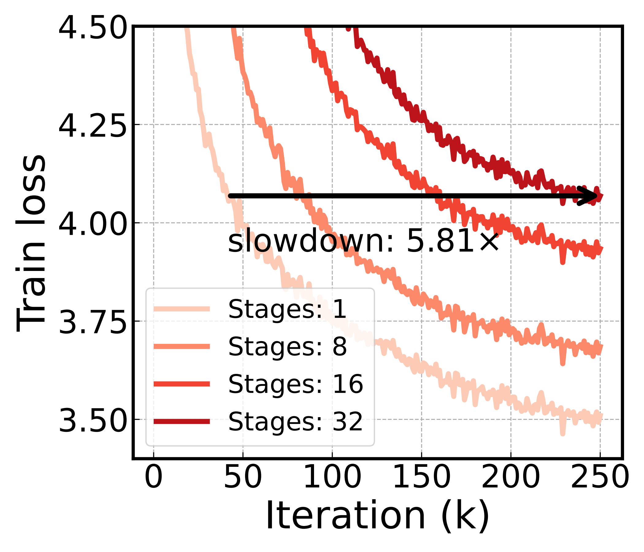
For instance, take a 95M-parameter Transformer, train it under asynchronous pipeline parallelism, and vary \(P\) from 1 to 32. The model, the data, the optimizer, the schedule — all held constant. Only the number of stages changes. At \(P{=}32\), training converges nearly six times more slowly than at \(P{=}1\).

§2Why delay hurts: oscillation under misalignment

To explain why delay hurts so much, it helps to recall what Adam actually does. Adam maintains a running estimate of the second moment of the gradient, \(V_t\), and rescales each coordinate of the update by \(\mathrm{diag}(V_t)^{-1/2}\). The effect is a per-coordinate learning rate: directions with large historical gradients are damped, directions with small ones amplified. When the loss curves much more steeply along some directions than others — as it does in Transformers [4][5] — this coordinate-wise adaptivity is what keeps the steep directions from oscillating and the shallow ones from stalling.

Yet this rests on a hidden assumption. Coordinate-wise adaptivity is only effective when the eigenvectors of the Hessian — the directions that matter for curvature — are close to coordinate directions. If the Hessian's eigenbasis is rotated away from the coordinate basis, Adam's rescaling, applied along the wrong axes, can no longer suppress oscillations along the dominant eigenvector — its effective adaptivity diminishes, and its trajectory begins to look like that of an optimizer without coordinate-wise adaptation.

This is where our key insight enters. Whether delay is damaging depends on how much the update directions oscillate: when the trajectory is smooth, stale gradients remain closely aligned with the current update, and delay is benign. When the trajectory oscillates, delayed gradients point in outdated or adversarial directions, actively opposing progress. The quadratic \(\min_w \tfrac{1}{2}w^\top H w\) makes this concrete.

When \(H\) is diagonal, AdaSGD — which applies a single learning rate uniformly across all coordinates — oscillates along the dominant eigenvector direction while progressing slowly along non-dominant ones. Adam, by contrast, yields a smooth, near-monotone trajectory toward the optimum. This smooth trajectory makes Adam robust to delay: as we show in the paper, when update directions are locally consistent (\(u_t \approx u\)) and gradient noise is small, the delayed trajectory \(\{\tilde{x}_t\}\) closely approximates the original trajectory \(\{x_t\}\) — introducing delay had negligible effect on convergence.

When \(H\) is non-diagonal — the same eigenvalues, but the eigenbasis rotated away from the coordinate axes — Adam's effective adaptivity diminishes. Its trajectory oscillates along the dominant eigenvector direction, looking very much like AdaSGD. In this case, delay is catastrophic: stale gradients point in adversarial directions relative to the current iterate, substantially degrading convergence.

Notice that \(\|H\|_{(1,1)}\), the sum of the magnitudes of the Hessian's entries, is smallest when the Hessian is diagonal and grows as the eigenbasis rotates away from the coordinate axes, acting as a proxy for basis misalignment. In the paper we turn this intuition into a convergence analysis: we show that how much delay slows training is governed by this misalignment. To focus on the core intuition for a general audience, we leave the precise assumptions and bound to the paper.

§3The remedy: optimize in a rotated basis

If misalignment is the catalyst that turns delay into a problem, the fix is to remove the misalignment. Staying in vector form for a moment: let \(\mathcal{U}\) be a rotation whose columns are the Hessian's eigenvectors, and run Adam not in the original coordinates but in the rotated ones \(\tilde{w} = \mathcal{U}^\top w\), projecting each step back afterwards. Written in the original space, the update is

The obstacle is \(\mathcal{U}\) itself. A single weight matrix \(W \in \mathbb{R}^{m\times n}\) flattens to a parameter vector \(w = \mathrm{vec}(W)\) of length \(mn\), so a full rotation \(\mathcal{U}\) is an \(mn \times mn\) object — impossible to store or diagonalize for any real layer. Two structural assumptions on the Hessian make it tractable. Block-diagonality, well supported empirically in Transformers [4][11], lets us rotate each weight matrix on its own rather than the whole parameter space at once. Kronecker factorization then splits the per-matrix rotation as \(\mathcal{U} = V \otimes U\), with a small \(U \in \mathbb{R}^{m\times m}\) for the rows and \(V \in \mathbb{R}^{n\times n}\) for the columns.

This is precisely why the rotation ends up on both sides of the matrix. Applying the Kronecker-factored rotation \(\mathcal{U} = V \otimes U\) to the flattened weights is, by the standard vec identity, the same as a two-sided product on the matrix:

Since the actual update runs at the matrix level, the update rule can be written as follows:

What should \(U\) and \(V\) be? We want them to diagonalize the Hessian, but the Hessian is out of reach, so we use its standard cheap surrogate — the empirical Fisher \(\mathbb{E}[g g^\top]\), \(g = \mathrm{vec}(G)\). Under the same Kronecker assumption this Fisher factors (up to a scalar) as \(\mathbb{E}[G^\top G] \otimes \mathbb{E}[G G^\top]\). A short calculation then shows that the eigenvectors of these two factors — \(U\) from \(\mathbb{E}[G G^\top]\), \(V\) from \(\mathbb{E}[G^\top G]\) — diagonalize the Hessian, aligning its eigenbasis with the coordinate axes.

Either way, both \(U\) and \(V\) are refreshed infrequently — once every ten optimization steps in our default configuration — using a single step of power iteration followed by a QR decomposition. The cost amortizes to a small fraction of training time.

§4Experiments

With the method in hand, the question is whether it works in practice. We present three experiments here — varying the pipeline depth, the model size, and the fidelity of the rotation. More results (GPU-hour efficiency, the Hessian's \((1,1)\)-norm shrinking under rotation, advanced-optimizer comparisons, and 3B-scale runs) are presented in the paper. Two metrics recur throughout: final training loss after a fixed iteration budget, and slowdown — the ratio of iterations needed to reach a target loss at a deep pipeline versus a single stage.

Deeper pipelines barely hurt anymore

First, we train identical 95M-parameter Transformers under asynchronous pipeline parallelism with varying \(P\) from 1 to 32. This changes how stale the gradients are.

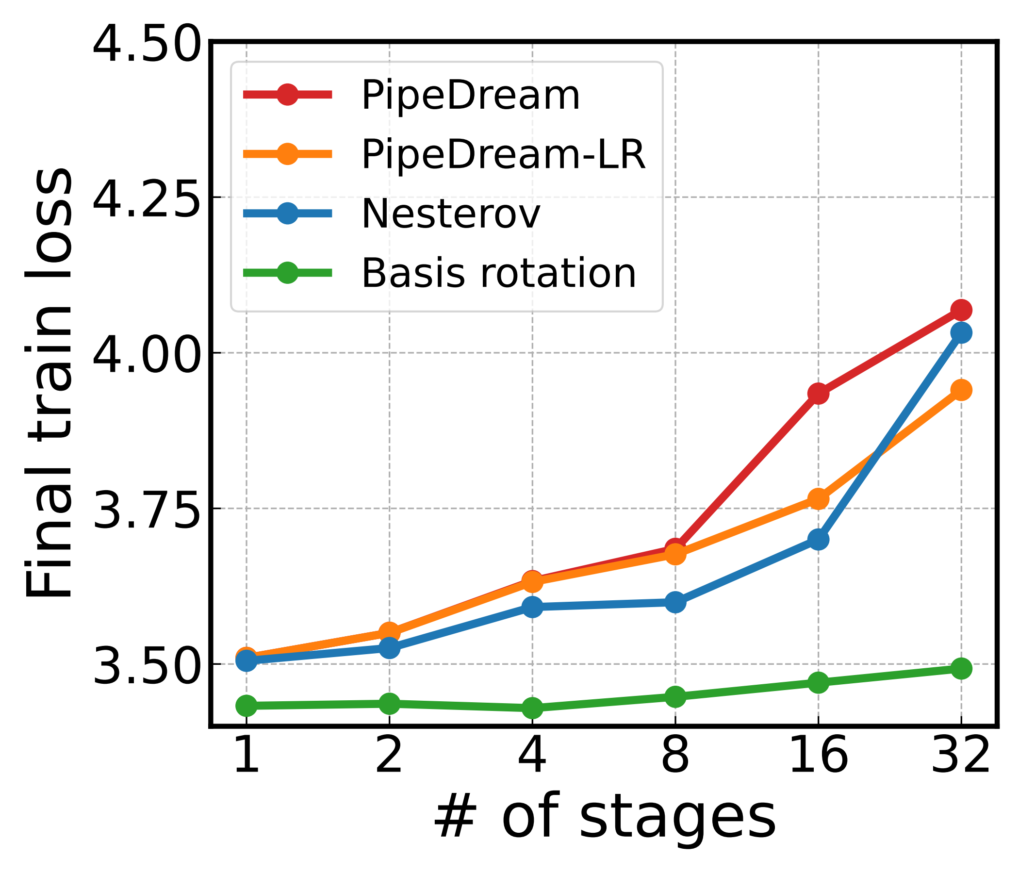
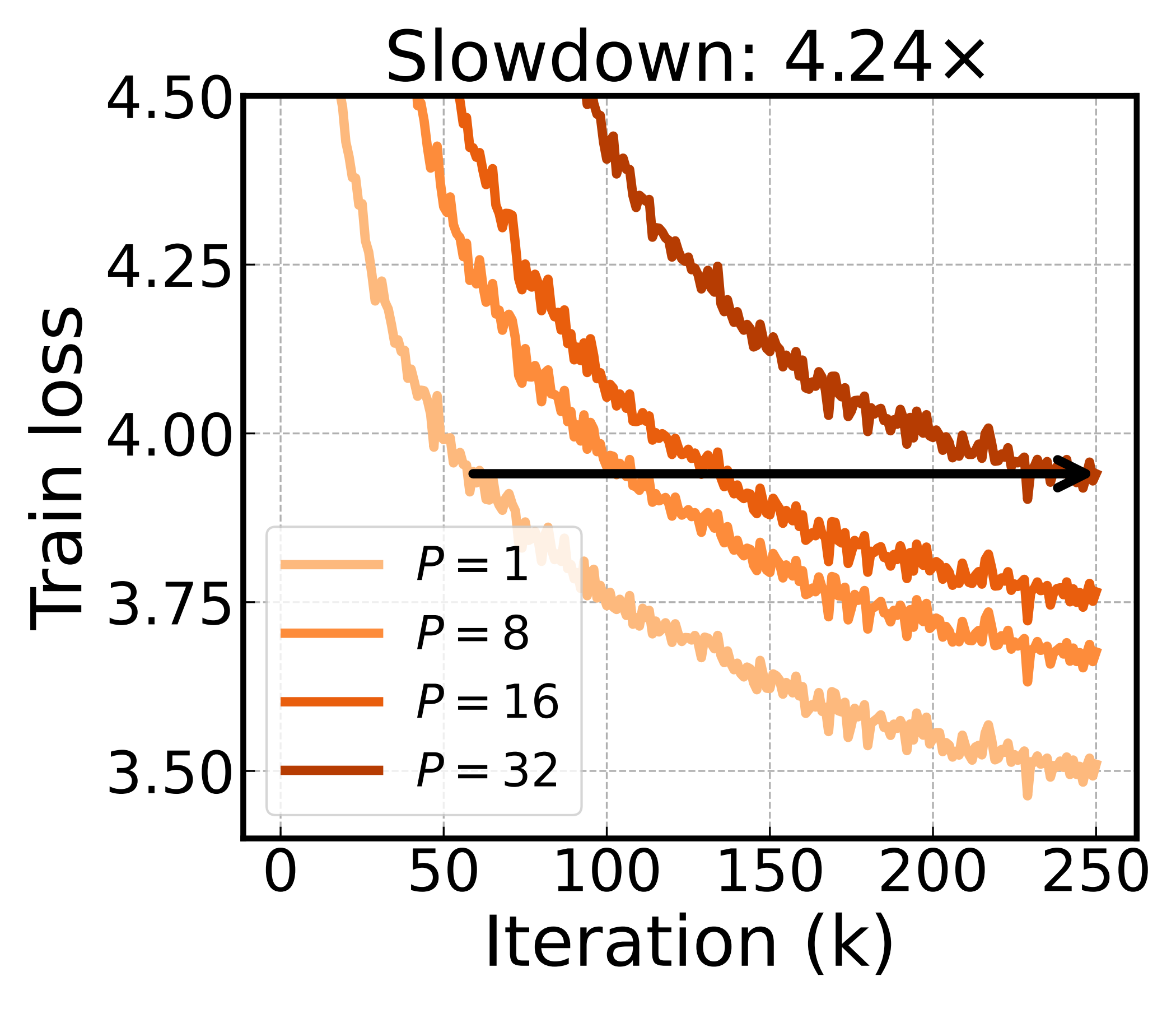
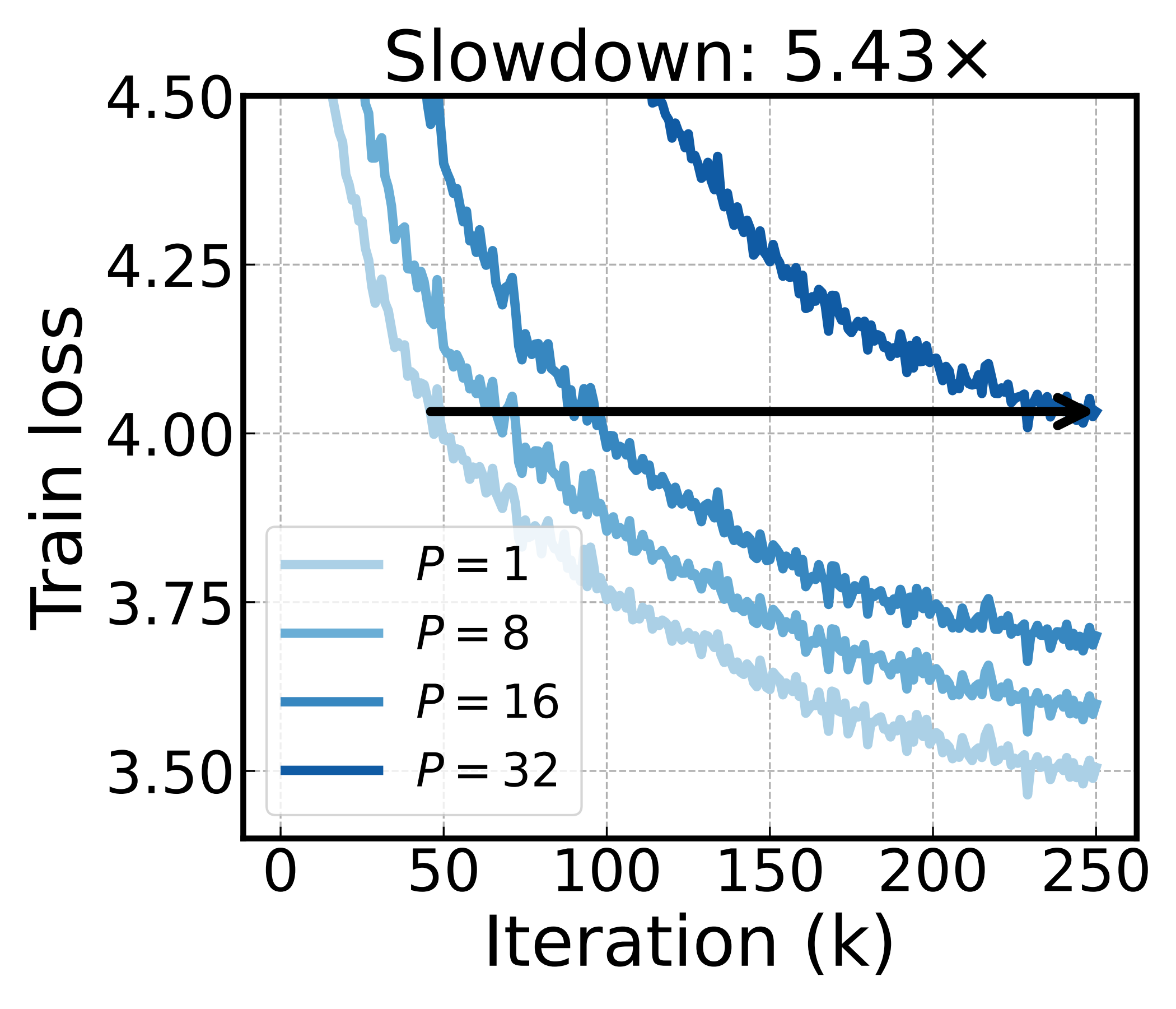
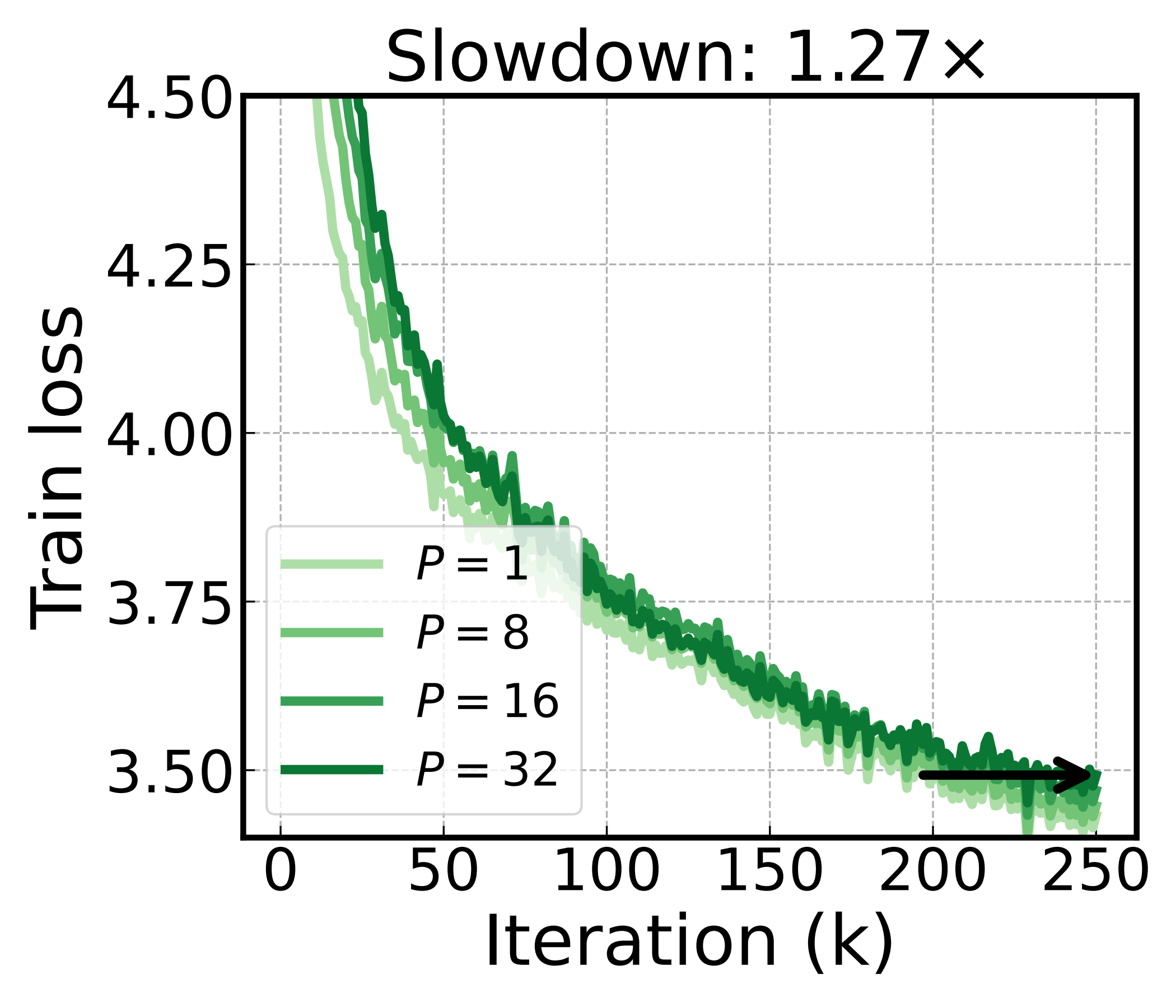
Basis rotation barely slows down as the pipeline deepens, while the baselines are hit hard. The best of them, PipeDream-LR, still needs 4.24× as many iterations at \(P{=}32\) as at \(P{=}1\) — basis rotation needs only 1.27×. The same depth that costs the baselines so much costs basis rotation almost nothing.

The advantage grows with model size

A important question is whether the benefit holds as the model gets bigger. We fix the pipeline at \(P{=}24\) and scale the embedding dimension to produce a 0.1B and a 1B model.

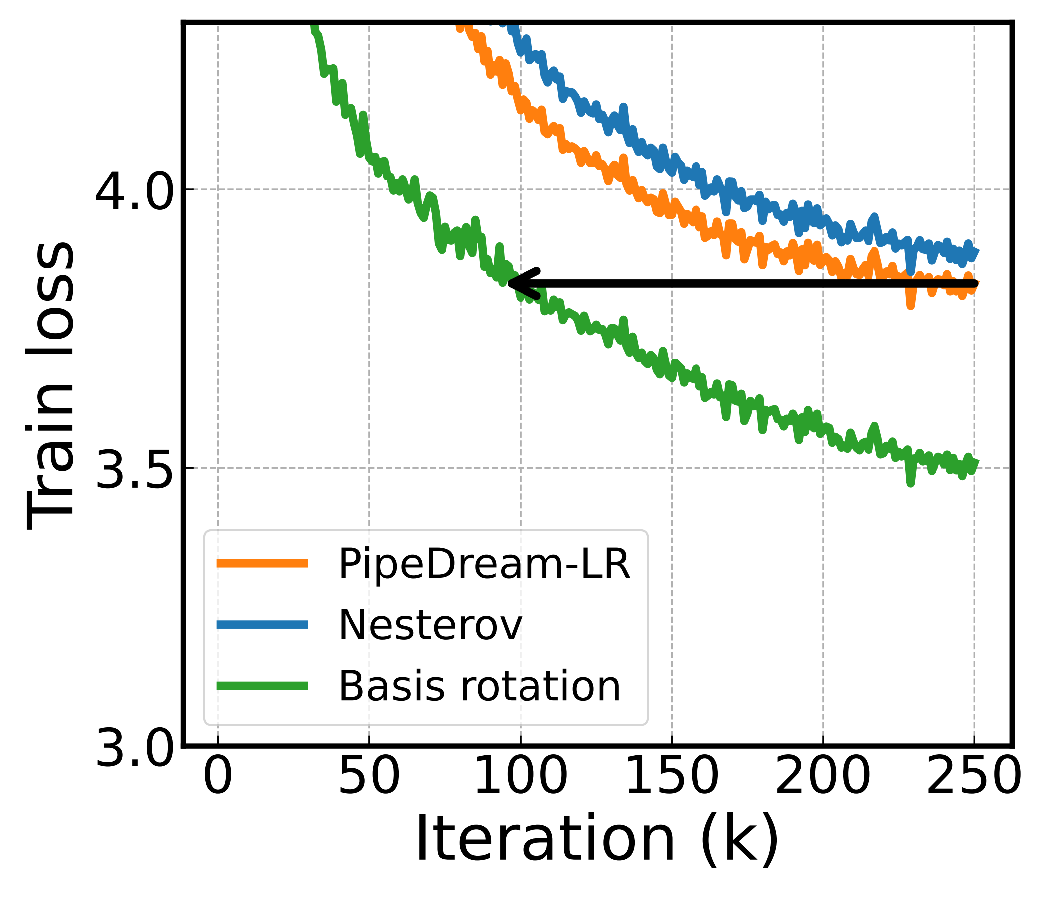
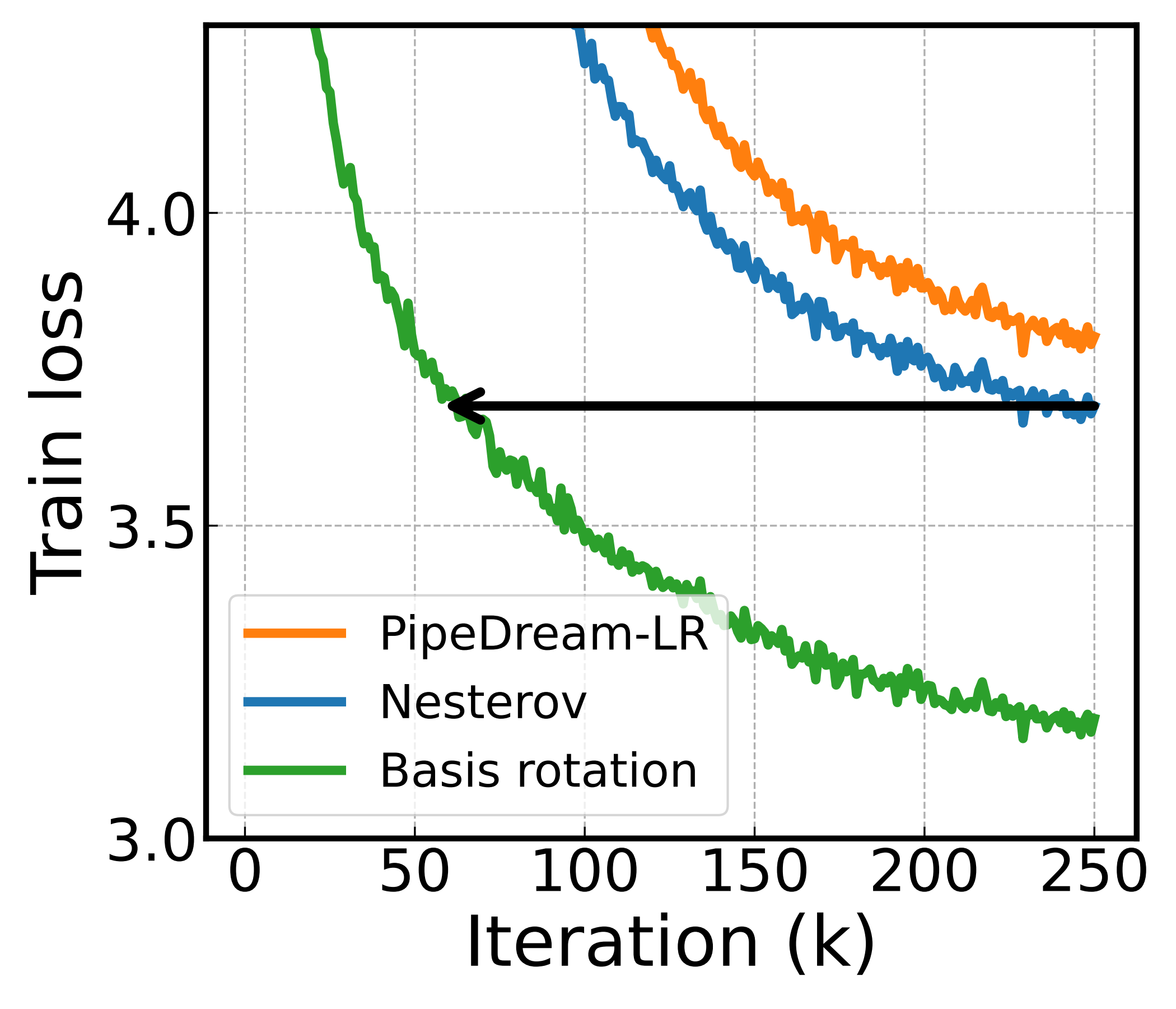
Here, only the model grows — the pipeline depth, and hence the raw delay \(\tau\), is held fixed. Figure 6 demonstrates the performance gap between basis rotation and the baselines widens for larger models. The iteration saving over the best baseline climbs from 62.4% at 0.1B to 76.8% at 1B.

Better alignment, more robustness

The rotation can be estimated from second moments (high fidelity) or reused from the momentum buffer (cheap), and applied on both sides of the weight matrix (bilateral) or only the smaller one (unilateral). The default we described — second-moment, bilateral — is the most accurate corner of this design space. The others trade fidelity for memory.

Method	S	G	Slowdown
PipeDream-LR	—	—	4.24×
Basis rotation	1st	Uni	2.55×
	1st	Bi	1.77×
	2nd	Uni	1.66×
	2nd	Bi	1.27×

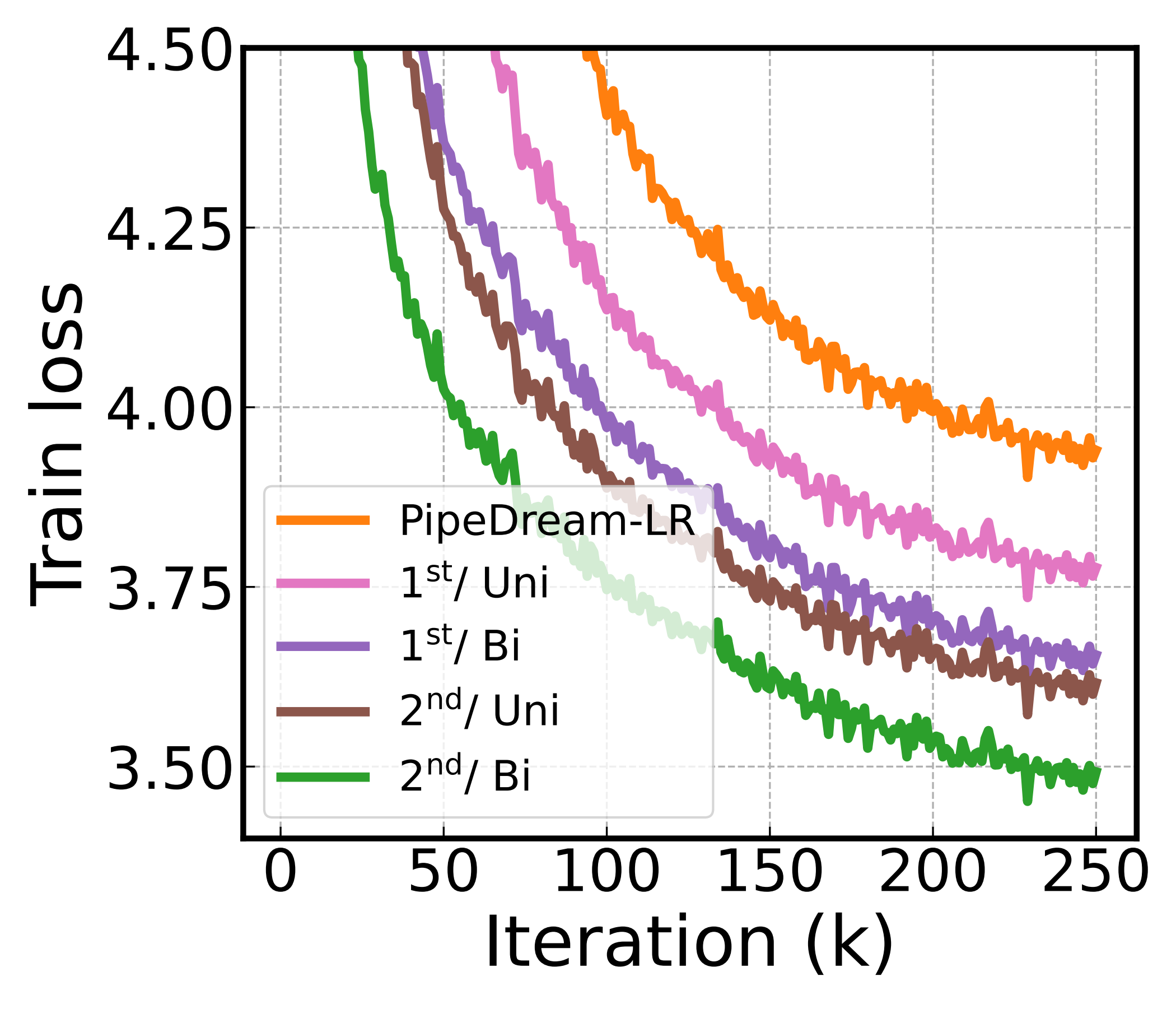
The ordering matches what the misalignment story predicts: second-moment beats first-moment, bilateral beats unilateral, and the most accurate combination is the most robust to delay. That monotonic relationship is the causal evidence — robustness tracks alignment fidelity. Moreover, even the cheapest variant (first-moment, unilateral) cuts the slowdown to 2.55×, comfortably below the best baseline's 4.24×.

§5Stage-aware rotation: spending the budget where it matters

Finally, we designed stage-aware rotation. The idea is simple: keep the total computation for subspace updates fixed, but skew it toward the earliest, highest-delay stages — refresh the early stages more often and the late ones less. This follows from the same misalignment picture: because the earliest stages carry the longest delay, they weigh most heavily on the effective, misalignment-weighted delay that governs convergence — so tightening their alignment is what helps the most.

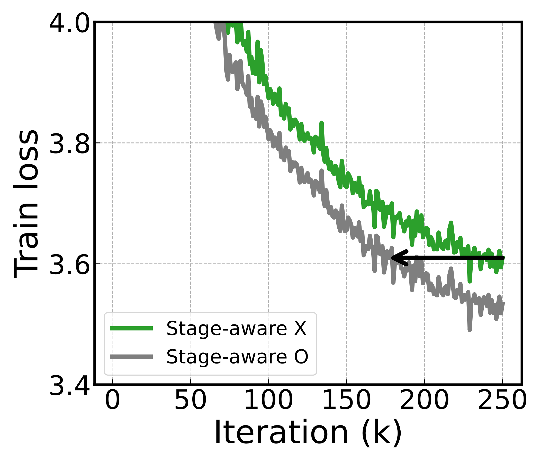
The result illustrates that with the budget reallocated this way, training reaches the same loss 29.2% faster than uniform allocation. The speedup confirms the theoretical insight from the stage-dependent convergence analysis.

§6Summary

Basis rotation effectively neutralizes the impact of delay, restoring scalable asynchronous training and unlocking a new regime for bubble-free execution at scale.

@inproceedings{jung2026mitigating,
  title={Mitigating Staleness in Asynchronous Pipeline Parallelism via Basis Rotation},
  author={Jung, Hyunji and Shin, Sungbin and Lee, Namhoon},
  booktitle={International Conference on Machine Learning},
  year={2026}
}

References

- [1] S. Rajbhandari, J. Rasley, O. Ruwase, Y. He. ZeRO: Memory Optimizations Toward Training Trillion Parameter Models. SC, 2020. arXiv:1910.02054
- [2] Y. Huang, Y. Cheng, A. Bapna, et al. GPipe: Efficient Training of Giant Neural Networks using Pipeline Parallelism. NeurIPS, 2019. arXiv:1811.06965
- [3] A. Harlap, D. Narayanan, A. Phanishayee, et al. PipeDream: Fast and Efficient Pipeline Parallel DNN Training. arXiv:1806.03377, 2018.
- [4] Y. Zhang, C. Chen, T. Ding, Z. Li, R. Sun, Z.-Q. Luo. Why Transformers Need Adam: A Hessian Perspective. NeurIPS, 2024. arXiv:2402.16788
- [5] J. Zhang, T. He, S. Sra, A. Jadbabaie. Why Gradient Clipping Accelerates Training: A Theoretical Justification for Adaptivity. ICLR, 2020. arXiv:1905.11881
- [6] S. Xie, M. A. Mohamadi, Z. Li. Adam Exploits ℓ∞-geometry of Loss Landscape via Coordinate-wise Adaptivity. ICLR, 2025. arXiv:2410.08198
- [7] N. Vyas, D. Morwani, R. Zhao, et al. SOAP: Improving and Stabilizing Shampoo using Adam. arXiv:2409.11321, 2024.
- [8] J. Zhao, Z. Zhang, B. Chen, et al. GaLore: Memory-Efficient LLM Training by Gradient Low-Rank Projection. ICML, 2024. arXiv:2403.03507
- [9] B. Yang, J. Zhang, J. Li, et al. PipeMare: Asynchronous Pipeline Parallel DNN Training. MLSys, 2021. arXiv:1910.05124
- [10] T. Ajanthan, S. Ramasinghe, Y. Zuo, G. Avraham, A. Long. Nesterov Method for Asynchronous Pipeline Parallel Optimization. ICML, 2025. arXiv:2505.01099
- [11] N. Abreu, N. Vyas, S. Kakade, D. Morwani. The Potential of Second-Order Optimization for LLMs: A Study with Full Gauss-Newton. ICLR, 2026. arXiv:2510.09378